STATISTICS

 STATISTICS

Statistics is the science of collecting, organizing and analyzing the data. Statistics is helpful in better decision making. It is of 2 types 

1)Descriptive Statistics

2)Inferential Statistics

Define Data?

        Data is nothing but the Facts & Pieces of information that can be measured.

1)Descriptive Statistics              

          Descriptive statistics is nothing but the Organizing the data ,Summarizing the data and Presenting the data in to an Informative Way.    

-->Descriptive statistics focus on describing the visible characteristics of a dataset (a population or sample).

2)Inferential Statistics

            It is a technique where in we use the data that we have measured to form conclusions. 

-->Inferential statistics make predictions about a larger dataset, based on a sample of those data.

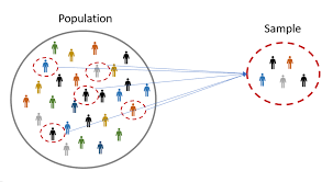
Population & Sample:-

-->A population is the entire group that you want to draw conclusions about. Population is denoted by N

-->A sample is the specific group that you will collect data from. The size of the sample(n) is always less than the total size of the population(N). Sample is denoted by n.

Different Sampling Techniques:-

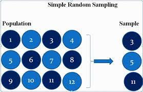
1)Simple Random Sampling:-

                  In Simple Random Sampling every number of the population(N) has an equal chances of being selected for your sample(n).

2)Stratified Sampling:-

           In Stratified Sampling the Population(N) is split into non-overlapping groups

             ex:- The Gender data is divided into 2 groups Male & Female.

3)Systematic Sampling:-

         Systematic Sampling is nothing but the from a population N we select every nth individual.

                     ex:- I am Conducting a survey on Covid in mall, i will select every 10th person i see for the survey, this is nothing but the Systematic Sampling.

4)Convenience Sampling:-

             Lets consider that i am doing a survey replating to specific topic for ex Library used by  Data scientist, the survey is conducted to people who are data scientist. This process is nothing but Convenience Sampling.

Variable: -

A variable is a property that can take on any value.

-->Their are two kinds of variables

           1)Quantitative Variable

                        Quantitative variables cam be measured numerically i.e. we can perform mathematical operations like add, subtract, multiply, divide etc. on Quantitative Variable                                   e.g. height, weight, or age

          2)Qualitative/Categorical Variable

                                   Categorical variables are those  variables in which the  data represent groups. On Qualitative variable we can perform rankings , classifications etc.

There are two types of quantitative variables: 

               1)Discrete  2)continuous.

Discrete

             The Quantitative discrete variables are variables which takes the values that can be  countable and have an finite number of possibilities. The values are mostly integer's but not always. The some of the examples of discrete variables are 

• Number of children per family
• Number of students in a class
• Number of citizens of a country

Continuous

          Quantitative continuous variables are variables  which takes the values that  are not countable. For example:

• Age
• Weight
• Height

Their are 4 types of Measured Variable:-

    1)Nominal Data

    2)Ordinal Data

    3)Interval Data

    4)Ratio Data

Nominal data: -

                Nominal data is nothing but the categorical data. For example, for preferred mode of transportation, we have the categories of car, bus, train etc.

Ordinal Data: -

     In ordinal data, order of the data matters but value does not matter.

In above figure, we can say that order of the data matters but not value i.e. quantity of the data.

Interval data:-

                     In Interval Data Order of the data matters, value of the data matters. Natural Zero is not present in Interval Data 

-->Interval data, also called an integer, is defined as a data type which is measured along a scale, in which each point is placed at equal distance from one another.

From above figure we can observe in Time column each point is differ by 15min.

Ratio Data: -

          Ratio data is nothing but the it classifies the data in to category and ranks the data.

Frequency Distribution: -

              Frequency Distribution is nothing the value count of the elements.

Bar Graph: -

         Bar Graph is drawn on the basic of Frequency Value. Bar graph works with discreate data. Bar graph is a graph that represents the categorical data with rectangular bars .The bars can be plotted as any one of the type like vertically or horizontally.

Histogram: -

                   Histogram works with continuous value. Similar in appearance to a bar graph.

Arithmetic Mean for Population and sample:-

                          Mean is nothing but the average. The mean of Population is given by the symbol 

μ.The mean of sample is given by X̄.

Sample Mean = $\frac{\sum x_i}{n}$ =$\frac{(x_1+x_2+x_3+\cdots +x_n)}{n}$

Where,

• $\sum x_i$ = sum of values of data
• n = number of values of data

       

   Population Mean (μ) = ∑X / N

           ∑X is the sum of data in X

           N is the count of data in X.

Central Tendency: -

                  It refers to the measure used to determine the center of the distribution of data. The central tendency measures are Mean, Median, Mode.  

-->Mean is nothing but the average that we discussed above. Mean will be affected by the outliers.

-->Median is nothing the middle value of the data. Median wont get affected by the outliers present in the data.

    for example:- consider the data 1,3,4,2,5,6,7,8,0

                   STEP1:- Sort the data in ascending order

                                     0,1,2,3,4,5,6,7,8

                   STEP2:- Find out the middle value 

                                     Median is 4.

-->Mode is nothing but the most repeated value in the data. Generally mode is used for replacing missing categorical data present in data. 

       foe example: Consider the data 1,2,4,5,6,7,5,8,5,3,1,2,5,4,5,6,8,9,0,1,3,5

                      Mode=Most repeated number=5

Measure of Dispersion:-

      Dispersion is nothing but the spread of the data.  It says how distributions are different from one another.

-->We can find the spread of the data in 2 ways

            1)Variance

            2)Standard Deviation

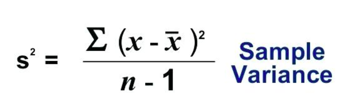
1)Variance:-

                Variance is of 2 types i.e. population variance & sample variance.

-->Population variance is denoted by .Sample variance is denoted by.
-->The formula to calculate population variance is 

-->The formula to calculate sample variance is 

-->Sample variance is divided by n-1 instead of N because out of the experimentation done by taking different sample from population and calculating variance of the sample collected they observed variance of population and sample are varying a lot. In order to overcome this sample variance is divided by n-1. n-1 is performed better when compared to n-2,n-3 .. etc.

2)Standard deviation:-

                     Standard deviation is nothing but the square root of the variance.

-->We probably prefer the standard deviation to represent the distribution of the data.

-->When the standard deviation is high, we can say that the data is more dispersed. When ever standard deviation is low we can conclude that the data is not more dispersed.

Five number summary:-

                  Five number summary is used to summarize the data.

-->By using this 5 number summary we will construct Box Plot. Box plot is nothing but the visualization way to find out the outliers. In 5 number summary we calculate

          1)Minimum

          2)First Quartile(Q1)

          3)Median

          4)Third Quartile(Q3)

          5)Maximum

-->After calculating above all 5 values we will calculate the lower fence & upper fence.

-->If the datapoints are below the lower fence & above the upper fence, then those data points are treated as outliers.

                 IQR=Inter Quartile Range=Q3 - Q1
                 Upper Fence=Q3 + 1.5*IQR

                 Lower Fence=Q1 - 1.5*IQR

-->The box plot is constructed as below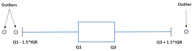

Lets discuss some of the distributions 

Gaussian/Normal Distribution: -

        Gaussian/Normal Distribution looks like a bell curve. In this distribution generally the center is mean, median, mode of the data. The area towards the left side of central line is similar to area towards the right side of central line.

Empirical formula:-

             Empirical rule is also called as 68-95-99.7% Rule i.e. with in the 1st standard deviation 68% of entire distribution present ,  with in the 2nd standard deviation 95% of entire distribution present and with in the 3rd standard deviation 99.7% of entire distribution present.

-->Some of the examples of data which follows normal distribution are height, weight, IRIS Dataset  etc.

Chebyshev's Inequality:-

              If variable belongs to Gaussian Distribution then we can say the distribution follows Empirical Rule.

-->If a variable does not belong to Gaussian Distribution, then use Chebyshev's Inequality principle to understand distribution of data.

-->With in the 1.5 Standard deviation , 56% of data present. With in the 2 Standard deviation 75% of data present. With in the 3 Standard deviation 89% of data present and with in the 4 Standard deviation 94% of data present. 

Z-Score:-

      Z-Score helps us to find out the value is how much standard deviation away from the mean. If we get z-score value as positive(+ve) then we can say the datapoint is present towards right side similarly vice-versa.

-->If we apply Z-Score formula to every datapoint present in the distribution. After applying Z-Score the distribution is converted into with the mean=0 & Standard deviation=1

-->The distribution with mean=0, Standard deviation=1 then this distribution is called as STANDARD NORMAL DISTRIBUTION 

Standardization:-

         The process of converting the distribution with mean=0 & standard deviation=1 is called Standardization. In standardization internally Z-Score formula is applied.

Normalization:-

       Normalization gives us the process where we can define the lower bound & upper bound and convert the distribution between lower bound & upper bound. 

-->MinMax scaler is used to convert the data into normalization.

click here to see practical part

P Value:-

       P value is nothing but the probability for the null hypothesis to be true.

-->Lets consider a space bar of a keyboard, we mostly touch on the middle of the space bar. If the P=0.8 i.e. out 0f 100 touches of spacebar, 80 times touched in the middle of the spacebar.

-->Lets understand the hypothesis testing, confidence interval, significance value by taking tossing a coin as example

-->We need to test whether the coin is a fair coin or not by performing 100 tosses.

    A coin is said to be fair, if we get P(H)=0.5, P(T)=0.5

Hypothesis Testing:-

1)Null Hypothesis:- Coin if fair

2)Alternate Hypothesis:- Coin is unfair

3)Experiment

4)Reject or Accept the null hypothesis

If the significance value is 0.05, usually significance value is given by domain experts. For significance value 0.05, the confidence Interval is 95%.

-->Out of 100 times tossed if we get 80 Heads then according to  95% confidence interval. The coin is fair. So, accept the null hypothesis & reject the alternate hypothesis.

PERFORMANCE METRICS:-

Performance metrics are used to find out how well our Model is working

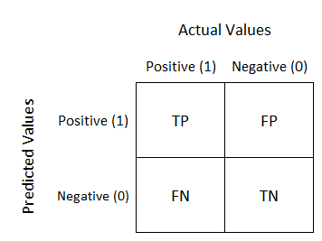
1)Confusion Matrix:-

                   A confusion matrix is used for evaluating the results of a classification machine learning model. 

where

TN(True Negatives) - model predicts negative outcomes and the real/known outcome is also negative

TP(True Positives) - Model predicts positive outcome and the real outcome is also positive  

FN(False Negatives) - model predicts negative outcome but known outcome is positive

FP(False Positives) - model predicts positive outcome but known outcome is negative

2)Type 1 Error:-

         Type 1 Error is nothing but the we reject the null hypothesis when in reality it is true. Type 1 Error is called FPR

3)Type 2 Error:-

           Type 2 Error is nothing but the we accept the null hypothesis when in reality it is False. Type 2 Error is called FNR.

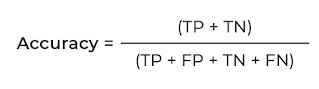
4)ACCURACY:--

                   Accuracy is the ratio of  Number of correct predictions to the Total number of predictions

-->Generally the result of accuracy is taken into consideration for Balanced data

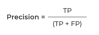
5)PRECISION:--

               Precision can be defined as out of total actual predicted positive values, how many values are actually positive is called Precision.

 

• Whenever FP is more important to reduce use Precision

                        eg:-In Spam classification, if we got spam mail it should be identified as spam & in spam classification we should concentrate on reducing FP i.e. even though the mail we got is not a spam but if our algorithm detects it as a spam, then we are going to miss our important mails .so in order to avoid this case we should concentrate on reducing FP

6)RECALL:--

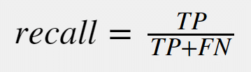
                Recall can be defined as out of total actual positive values, how many values did we correctly predicted positive is called Recall.

• When ever FN is more important to reduce use Recall

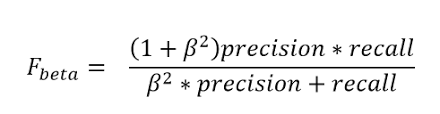
                             eg:-In classifying a person whether we has cancer or not FN is more important to reduce. If our model predicts that a person don't have a cancer even though  he has a cancer this leads to increase of cancer cells in his body & affects his health.

7)F-BETA:--

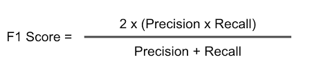
            The F-beta score is nothing but the weighted harmonic mean of precision and recall.

->When ever if we want to reduce both FP & FN  use β=1.It is also called as F1 Score

-->When ever FP is more important to reduce use β=0.5

• F0.5-Measure = ((1 + 0.5^2) * Precision * Recall) / (0.5^2 * Precision + Recall)
• F0.5-Measure = (1.25 * Precision * Recall) / (0.25 * Precision + Recall)

-->when ever FN is more important to reduce use β=2

• F2-Measure = ((1 + 2^2) * Precision * Recall) / (2^2 * Precision + Recall)
• F2-Measure = (5 * Precision * Recall) / (4 * Precision + Recall)

CO-VARIANCE:-

         Covariance is nothing but the measure of relationship between two random variable.

  EX:- Height & weight of a person i.e. if height of a person increases , weight of that person also increases

-->If one variable is increasing & another  variable also increasing its value means we can those two variables has positive co-variance.

-->If one variable is increasing & another variable decreasing means we can say those two variables has negative co-variance.

-->The major disadvantage of covariance is covariance says whether variables are positively corelated or negatively corelated but as the covariance value is not limited to certain limits we cannot say how much two variables are positively co related or how much negatively co related.

Pearson correlation coefficient:-

        Pearson correlation coefficient it basically restricts the value between -1 to 1.The more towards +1 means more positively corelated. The near value towards -1 means negatively corelated.

 
From above graph we can say that 

1. If all points fall on same line & line moving downwards we can say it is the perfect example of negative correlation.ρ=-1
2. If all the points fall around the line and the line is decreasing means we can say it is also as negative correlation. The value of Pearson correlation lies between -1 to 0. 
3. If the point lie around the line & if the line moving upwards then we say it as positive correlation .The value of Pearson correlation lies between 0 to +1. 
4. If the point lie  the line & if the line moving upwards then we say it as perfectly positive correlation .The value of Pearson correlation is +1. 
5. If the values are randomly distributed then we say that it as no co relation. The value of correlation is 0.

-->Pearson correlation coefficient catches the linear property of variables very well.

Spearman's rank correlation coefficient:-

                   Spearman's rank correlation catches the non linearity property of variables also. In order to obtain this Spearman's rank correlation uses the rank of the variable.

-->Generally rank is calculated as above i.e. for Rank of IQ, Rank IQ=1 for higher value of IQ similarly this process continues. In this way based on the value present in the column Rank is calculated and substituted in below formula

Log-normal distribution: -

                              If y follows the lognormal distribution, then log(y) follows the Normal Distribution.

-->

Bernoulli's Distribution:-

                         Bernoulli Distribution has two outcomes either 0 or 1.

Three examples of Bernoulli distribution:

  ${\displaystyle P(x=0)=0{.}2}$ and ${\displaystyle P(x=1)=0{.}8}$

  ${\displaystyle P(x=0)=0{.}8}$ and ${\displaystyle P(x=1)=0{.}2}$

  ${\displaystyle P(x=0)=0{.}5}$ and ${\displaystyle P(x=1)=0{.}5}$

Binominal Distribution:-

                           Binominal Distribution is the combination of multiple Bernoulli Distribution.

Power Law Distribution:-

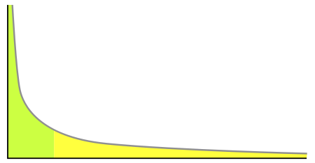
         Power law distribution is also known as 80-20 Rule.

Example of Power Law distribution is wealth distribution i.e. 80% of the wealth is present at 20% of population. Remaining 20% of wealth is present at the 80% population

-->If we draw a graph of wealth distribution it looks like   

Above graph is the example power-law graph, to the right has a long tail and to the left it has small tail. It also known as the 80–20 rule.

Central Limit Theorem:-

                         Taking the entire population into consideration to draw conclusion is not possible because of time, huge data. So, we generally  consider small amount of sample of data, but taking the the sample & performing the operations on sample and assuming the result will be applicable to entire population data is wrong.

   So, according to central limit theorem we will collect multiple samples of small size, then we perform certain operations on multiple sample data that we want to do. Then maximum or mean of multiple sample data result is taken into consideration by assuming this result will be applicable population data.

For example, if you want to calculate the mean of population(N), multiple samples(n1,n1,..) of data is collected and then mean is calculated on sample data's that we taken. Finally the mean of sample mean is taken into consideration as Population Mean.